Understanding Regularization Through Gradient Descent

Regularization is often introduced as a collection of techniques—L1, L2, dropout, early stopping, and so on.

That presentation makes it easy to memorize what regularization does without understanding why it works.

A better way to understand it is to start from a sequence of questions:

What is gradient descent actually doing?
What does the gradient tell us?
Why might a neural network’s weights become problematic?
How can we encourage the network to learn less sensitive solutions?
How does L2 regularization actually change gradient descent?
Why does dropout help?

This post follows that chain.

Start with Gradient Descent

Suppose we have a simple loss function:

$$J(x)=(x-3{)}^2$$

We want to find the value of $x$ that minimizes $J$.

The derivative is:

$$\frac{dJ}{dx}=2x-6$$

Gradient descent updates $x$ according to:

$$x_{\text{new}}=x-\alpha \frac{dJ}{dx}$$

where:

• $x$ is the current parameter
• $\alpha$ is the learning rate
• $\frac{dJ}{dx}$ is the gradient

What does the gradient tell us?

The gradient tells us how the loss changes if we change the parameter.

If the slope is positive:

$$\frac{dJ}{dx}>0$$

then increasing $x$ increases the loss. Therefore, to reduce the loss, we should decrease $x$.

If the slope is negative:

$$\frac{dJ}{dx}<0$$

then increasing $x$ decreases the loss. Therefore, we should increase $x$.

This is why:

$$x\leftarrow x-\alpha \frac{dJ}{dx}$$

works.

A Small Numerical Example

Take:

alpha = 0.1
x = 4

for i in range(1, 10):
    dx = 2 * x - 6
    x = x - (alpha * dx)

    print(f"iteration: {i}, dx: {dx}, x: {x}")

The updates are approximately:

$$4\to 3.8\to 3.64\to 3.512\to \cdots$$

The parameter approaches:

$$x=3$$

At $x=3$:

$$\frac{dJ}{dx}=0$$

The slope has become flat.

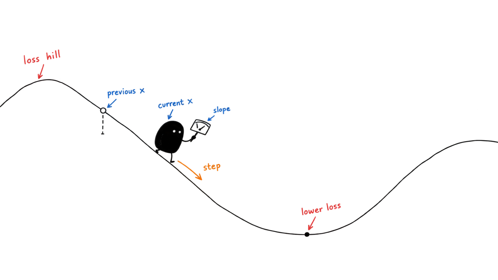
Gradient descent uses the local slope at the current point to decide the next step toward lower loss.

Important distinction

It is tempting to say:

“The goal of gradient descent is to find where the gradient is zero.”

A more accurate statement is:

The goal is to find parameter values that minimize the loss, using the gradient to guide the updates.

A zero gradient can occur at points that are not minima, so “gradient = 0” is a consequence of reaching a smooth minimum, not the fundamental definition of the goal.

Bring This Into a Neural Network

Now replace $x$ with a neural-network weight $w$.

A neuron might calculate:

$$z=w_1{x}_1+w_2{x}_2+b$$

The network eventually produces a prediction $\hat{y}$, and the loss function measures how far that prediction is from the true target.

So the training process is trying to find values of $W$ and $b$ that minimize:

$$J(W,b)$$

For one particular weight $w$, gradient descent looks like:

$$w\leftarrow w-\alpha \frac{\partial J}{\partial w}$$

What does $\frac{\partial J}{\partial w}$ mean?

It means:

If I slightly change this particular weight, how does the loss change?

That is the neural-network version of “slope.”

What Does a Weight Actually Do?

Consider:

$$z=w_1{x}_1+w_2{x}_2+b$$

Suppose:

$$x_1=2,w_1=3$$

Then $x_1$‘s contribution to $z$ is:

$$w_1{x}_1=6$$

If instead:

$$w_1=10$$

the contribution becomes:

$$20$$

So the weight controls how strongly that input influences the neuron’s pre-activation.

More precisely:

$$\frac{\partial z}{\partial x_1}=w_1$$

Therefore:

The magnitude of the weight tells us how sensitive $z$ is to that input.

A large positive weight means a strong positive influence.

A large negative weight means a strong negative influence.

A weight near zero means little direct influence.

The Regularization Question

This leads to the important question:

What happens if a neural network learns very large weights?

Imagine:

$$z=20x_1+x_2+b$$

The network is now extremely sensitive to $x_1$.

A tiny change in $x_1$ can produce a relatively large change in $z$.

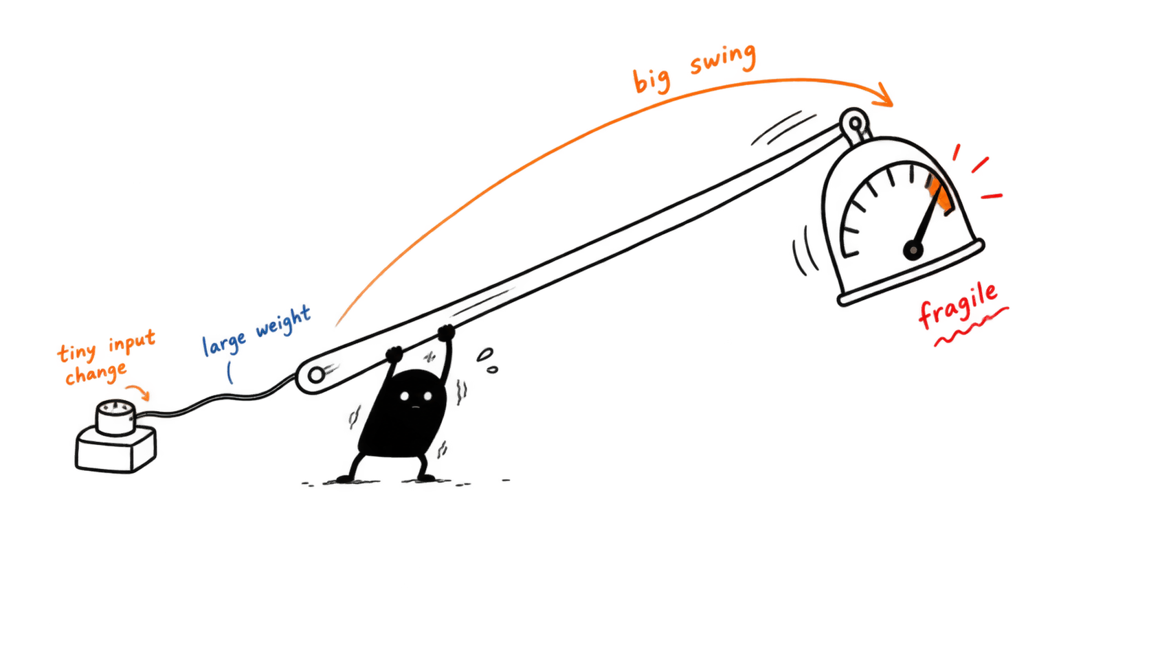
Large weights can turn small input changes into large output changes, which makes the learned behavior more fragile.

This can become problematic when the network starts relying heavily on patterns that are specific to the training data.

For example, suppose a training dataset contains some accidental relationship between $x_1$ and the target.

A sufficiently flexible network may exploit that relationship.

It can achieve excellent training performance while learning something that does not generalize well to new examples.

This is one way overfitting can arise.

So we can ask:

Can we encourage the network to use less extreme weights?

That is where regularization begins.

What Does “Regularization” Mean?

Regularization is not one particular algorithm.

It is a family of techniques that constrain the learning process to encourage better generalization.

The basic idea is:

Don’t allow the model to freely choose any solution that fits the training data. Prefer solutions with some desirable property.

Different regularization techniques constrain different things.

Technique	What is constrained?
L2	Weight magnitude
L1	Weight magnitude, with a tendency toward exact zeros
Dropout	Dependence on particular neurons/pathways
Early stopping	How long the model is allowed to specialize

The common idea is:

What aspect of the model could become unnecessarily specialized to the training data?

How Do We Tell the Optimizer What We Prefer?

Suppose two neural networks fit the training data reasonably well.

One has relatively small weights:

$$W=[2,1,3]$$

Another has much larger weights:

$$W=[20,1,30]$$

Suppose their training losses are:

$$J_A=0.10$$

and:

$$J_B=0.08$$

Without regularization, Model B looks better because its training loss is lower.

But we might prefer Model A because it uses less extreme parameters.

How do we communicate that preference to gradient descent?

We modify the objective function:

$$J_{\text{regularized}}=J_{\text{data}}+\text{penalty}$$

Now the optimizer isn’t merely asking:

“Which model fits the training data best?”

It is asking:

“Which model fits the data well while also satisfying my preference for a constrained solution?”

This is the central mechanism behind regularization.

L2 Regularization

For L2 regularization, we penalize the squared magnitude of the weights.

For a simple set of weights:

$$W=[2,3,-4]$$

the squared penalty is:

$$2^2+3^2+(-4{)}^2=29$$

The regularized objective becomes:

$$J_{\text{reg}}=J_{\text{data}}+\lambda \sum _i{w}_i^2$$

where $\lambda$ controls how strongly we care about the penalty.

Why square the weights?

Consider:

$$w_1=2$$

and:

$$w_2=10$$

Their penalties are:

$$2^2=4$$

and:

$$10^2=100$$

A weight of $10$ is only 5 times larger than a weight of $2$, but its squared penalty is 25 times larger.

Therefore, L2 strongly discourages very large weights.

Why Does L2 Actually Reduce the Weights?

This is where L2 connects directly back to gradient descent.

We have:

$$J_{\text{reg}}=J_{\text{data}}+\lambda w^2$$

Take the derivative:

$$\frac{\partial J_{\text{reg}}}{\partial w}=\frac{\partial J_{\text{data}}}{\partial w}+2\lambda w$$

The new term is:

$$2\lambda w$$

This is the important part.

If $w>0$:

$$2\lambda w>0$$

Gradient descent subtracts this positive quantity, pushing $w$ downward.

If $w<0$:

$$2\lambda w<0$$

Gradient descent subtracts a negative quantity, pushing $w$ upward.

Therefore, in both cases, L2 creates a force pulling the weight toward zero.

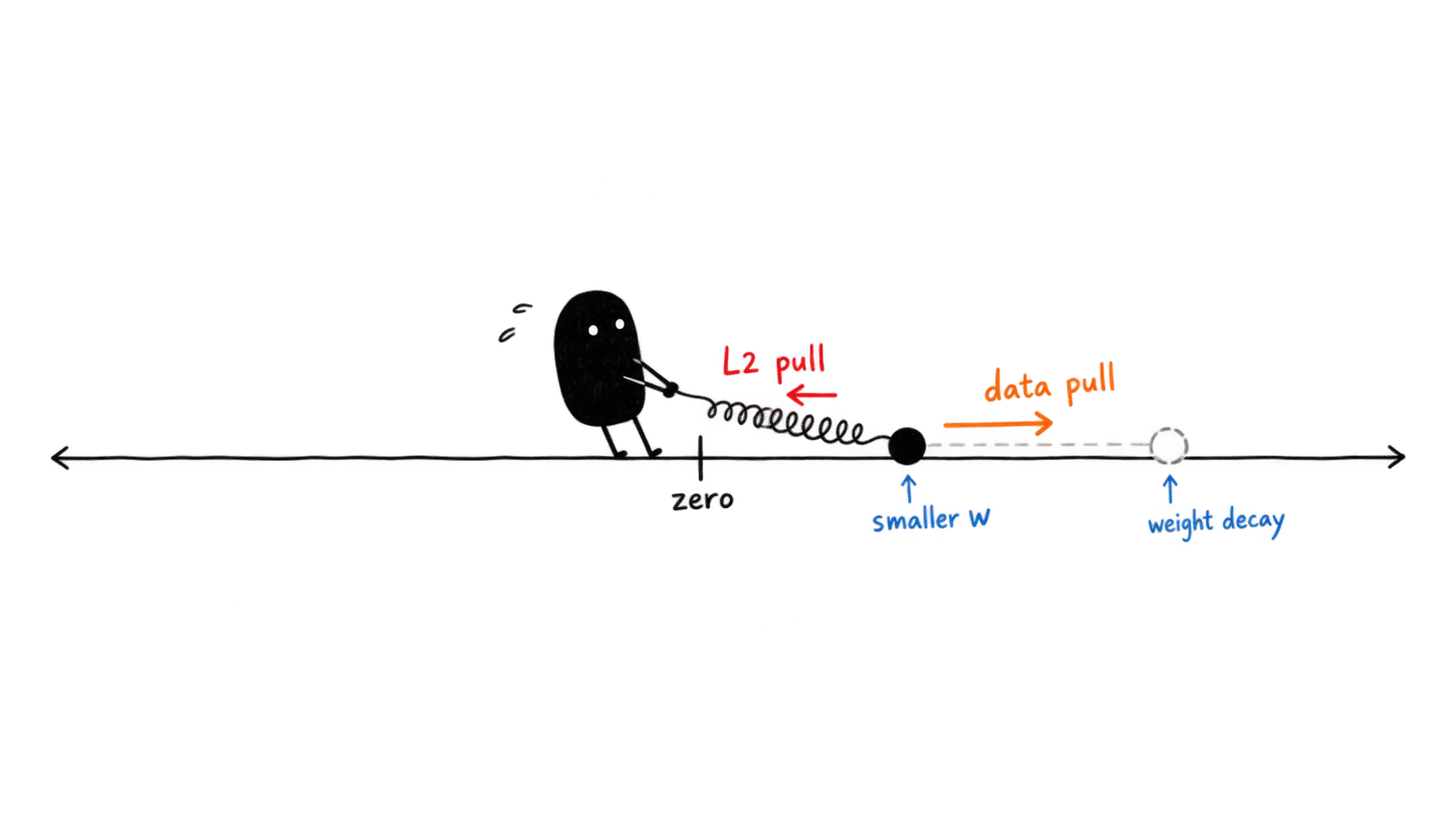
L2 adds a second pressure to the update: the data gradient still tries to improve predictions, while weight decay pulls the parameter toward zero.

Ignoring the ordinary data gradient for a moment:

$$w\leftarrow w-\alpha (2\lambda w)$$

which can be written as:

$$w\leftarrow (1-2\alpha \lambda )w$$

This is why L2 is often associated with weight decay.

A Concrete L2 Update

Suppose:

$$w=10,\alpha =0.01,\lambda =0.1$$

Ignoring the ordinary data gradient:

$$w_{\text{new}}=(1-2(0.01)(0.1))(10)$$

Therefore:

$$w_{\text{new}}=9.98$$

The weight has moved slightly toward zero.

If instead:

$$w=-10$$

then:

$$w_{\text{new}}=-9.98$$

Again, it moves toward zero.

The actual neural-network update includes both effects:

Data-loss gradient
        ↓
"Move the weight to improve predictions"

L2 gradient
        ↓
"Pull the weight toward zero"

So the learned weight is the result of balancing these two pressures.

Why Does Making the Weights Smaller Help?

Now connect the mathematics back to the neural network.

Recall:

$$z=w_1{x}_1+w_2{x}_2+\cdots +b$$

and:

$$\frac{\partial z}{\partial x_i}=w_i$$

Suppose:

$$w_1=20$$

The neuron is highly sensitive to $x_1$.

If L2 reduces it to:

$$w_1=2$$

then the same change in $x_1$ has much less influence on $z$.

So the conceptual chain is:

L2
 ↓
smaller weights
 ↓
less sensitivity to individual inputs
 ↓
less reliance on extreme parameter values
 ↓
more constrained model
 ↓
potentially better generalization

This is the connection between weight magnitude and overfitting.

Important qualification

Smaller weights do not automatically mean less overfitting in every situation.

If regularization is too strong, the network may lose too much flexibility and underfit.

The goal is not:

“Make every weight as small as possible.”

The goal is:

Find a balance between fitting the data and constraining the model.

What Does $\lambda$ Control?

Recall:

$$J_{\text{reg}}=J_{\text{data}}+\lambda \sum _i{w}_i^2$$

$\lambda$ determines the strength of regularization.

Small $\lambda$

For example:

$$\lambda =0.001$$

The regularization penalty contributes relatively little.

Gradient descent mainly focuses on fitting the training data.

Small λ
   ↓
Weak regularization
   ↓
Weights can remain relatively large
   ↓
More flexibility
   ↓
Potentially more overfitting

Large $\lambda$

For example:

$$\lambda =10$$

Large weights become much more costly.

Large λ
   ↓
Strong regularization
   ↓
Weights strongly pulled toward zero
   ↓
Less flexibility
   ↓
Potentially more underfitting

So:

$$\boxed{\lambda =\text{strength of the regularization pressure}}$$

Dropout: A Different Kind of Regularization

L2 constrains weight magnitude.

Dropout approaches the problem differently.

Ask:

What if the network is becoming too dependent on particular neurons?

Consider a hidden layer:

x₁ ─────→ h₁ ──────┐
x₂ ─────→ h₂ ──────┤
x₃ ─────→ h₃ ──────┼──→ next layer
x₄ ─────→ h₄ ──────┤
x₅ ─────→ h₅ ──────┘

During one training iteration, dropout might randomly remove $h_2$ and $h_4$:

x₁ ─────→ h₁ ──────┐
x₂ ─────→ ✕        │
x₃ ─────→ h₃ ──────┼──→ next layer
x₄ ─────→ ✕        │
x₅ ─────→ h₅ ──────┘

For that iteration, the next layer receives no contribution from $h_2$ and $h_4$.

On another iteration, a different subset may be removed.

The network therefore repeatedly has to make predictions using different subsets of its neurons.

This discourages it from becoming excessively dependent on one particular neuron or pathway.

Why Does Dropout Make Learning Harder?

Suppose the network normally has five hidden neurons:

h₁  h₂  h₃  h₄  h₅

With dropout, one iteration might use:

h₁  ✕  h₃  ✕  h₅

Another:

✕  h₂  h₃  h₄  ✕

Another:

h₁  h₂  ✕  h₄  h₅

So every training iteration is effectively working with a different subset of the network.

Yes, this makes each individual training step harder.

That is the trade-off.

The purpose is not to make training easier.

The purpose is to prevent the network from becoming too dependent on a particular internal pathway.

What Happens During Inference?

During prediction, we normally do not randomly drop neurons.

We want the full network to participate:

Training:
some neurons removed

Inference:
all neurons active

But this creates a scaling problem.

Suppose a neuron produces:

$$a=10$$

and the keep probability is:

$$p=0.5$$

Without scaling, dropout produces approximately:

50% of the time → 10
50% of the time → 0

Therefore the expected activation is:

$$E[a_{\text{dropout}}]=0.5(10)+0.5(0)=5$$

The average activation has been cut in half.

To compensate, we divide the surviving activation by the keep probability:

$$a\leftarrow \frac{a\odot d}{p}$$

So when the neuron survives:

$$\frac{10}{0.5}=20$$

Now the expected activation becomes:

$$0.5(20)+0.5(0)=10$$

which matches the original activation.

This is the idea behind inverted dropout.

The important point is:

The scaling keeps the expected activation aligned with the activation of the original network.

L2 vs Dropout

At this point, the distinction becomes much clearer.

	L2	Dropout
What is constrained?	Weight magnitude	Dependence on neurons/pathways
Main mechanism	Add weight penalty	Randomly remove neurons during training
Effect on weights	Pulls them toward zero	Indirectly discourages dependence
Training	Full network	Random subnetworks
Inference	Full network	Full network
Main intuition	Avoid extreme parameters	Avoid fragile internal dependencies

Both are regularization methods, but they attack the problem differently.

The Entire Conceptual Chain

The whole discussion can now be reconstructed from one question:

Why do we need regularization?

Because a neural network can become too specialized to its training data.

That leads to:

Overfitting
    ↓
Can we constrain the model?
    ↓
Regularization
    ↓
What should we constrain?
    ├── Weight magnitude → L2 / L1
    ├── Neuron dependence → Dropout
    └── Training duration → Early stopping

For L2:

Large weights
    ↓
Add λ * Σw² to loss
    ↓
Gradient changes
    ↓
Extra term 2λw
    ↓
Gradient descent pulls weights toward zero
    ↓
Less extreme parameterization
    ↓
Potentially better generalization

The key connection to gradient descent is:

The regularization term isn’t merely making the loss numerically larger.

It changes the gradient, and therefore changes how gradient descent moves through parameter space.

That is the deeper reason regularization works.

Final Mental Model

If there is one thing to retain, it is this:

Gradient descent asks: “Which way should I move the parameters to reduce the loss?”

Regularization modifies that question:

“Which way should I move the parameters to reduce the loss while also respecting a preference for simpler or less dependent solutions?”

L2 expresses that preference through a penalty on large weights.

Dropout expresses it by repeatedly forcing the network to function without randomly selected neurons.

The methods are different, but the underlying idea is the same:

Don’t merely fit the training data. Constrain how the network is allowed to fit it.