Reproducing Sequence-to-Sequence Learning: From LSTM Gates to Neural Machine Translation

The Problem

How can one model transform a variable-length English sentence into a different-length French sentence without aligning every input token to an output token by hand?

A conventional fixed-input classifier does not fit this problem. The input and output lengths vary, their vocabularies differ, and the useful information in an early source token may need to survive many recurrent steps before decoding begins. The 2014 sequence-to-sequence paper addressed this with two recurrent networks: an encoder compresses the source into recurrent state, and a decoder generates the target from that state.

This project reproduces that mechanism at practical scale. It does not claim to reproduce the paper’s WMT14 translation quality. The executed study uses 2,400 English–French sentence pairs, a one-layer model, 48-dimensional embeddings, 64 hidden units, and 16 CPU epochs.

Why This Approach?

The architectural question is more useful than treating translation as a black-box API call: can a recurrent state carry enough information for a second network to generate a complete sequence?

An LSTM was appropriate because its cell state provides an additive path through time. For one step, the gates are

f_{t} = σ (W_{f} [x_{t}, h_{t - 1}] + b_{f}), i_{t} = σ (W_{i} [x_{t}, h_{t - 1}] + b_{i})

g_{t} = tanh (W_{g} [x_{t}, h_{t - 1}] + b_{g}), o_{t} = σ (W_{o} [x_{t}, h_{t - 1}] + b_{o})

and the state update is

c_{t} = f_{t} ⊙ c_{t - 1} + i_{t} ⊙ g_{t}, h_{t} = o_{t} ⊙ tanh (c_{t}) .

For a single scalar cell, if $f_{t} = 0.9$ , the previous cell is $0.7$ , $i_{t} = 0.2$ , and the candidate is $0.5$ , then $c_{t} = 0.9 (0.7) + 0.2 (0.5) = 0.73$ . The forget path preserves most of the old value while the input path writes a smaller update. That controlled additive update is the key mechanism the implementation exposes.

Architecture

The encoder embeds each source token and runs a stacked, no-peephole LSTM over the sequence. Its final hidden and cell states initialize the decoder. The decoder starts with a start-of-sequence token and predicts a distribution over the target vocabulary at each step.

English tokens → encoder embeddings → encoder LSTM
                                      │ final (h, c)
                                      ▼
French <SOS> → decoder embeddings → decoder LSTM → vocabulary logits

The context is not a separate attention matrix. It is the complete set of final encoder hidden and cell states transferred to the decoder. That fixed-state bottleneck is faithful to the broad pre-attention design while the implemented no-peephole cell is a documented simplification.

During training, masked teacher forcing supplies the known previous target token where configured. During inference, the decoder must consume its own prediction. This mismatch is one reason a low training loss does not guarantee robust autoregressive translation.

Implementation

The repository separates two goals that are easy to conflate:

lstm_numpy.py computes the recurrent forward pass explicitly with NumPy.
The end-to-end encoder–decoder is implemented with explicit PyTorch gate equations, while PyTorch autograd performs backpropagation through time.

No prebuilt nn.LSTM, attention layer, Transformer, or pretrained embedding is used. The explicit gate implementation keeps tensor shapes and state transfer inspectable without requiring a hand-written production training engine.

The project verifies the math with finite differences. For parameter $θ_{i}$ , a numerical derivative is approximated by

\frac{\partial L}{\partial θ _{i}} \approx \frac{L ( θ _{i} + ϵ ) - L ( θ _{i} - ϵ )}{2 ϵ} .

Those estimates are compared with recurrent gradients. NumPy and PyTorch forward outputs are also checked for parity. The published suite contains 51 passing tests covering gates, recurrent gradients, padding, stacked encoders, teacher forcing, clipping, checkpoint resume, device behavior, and search correctness.

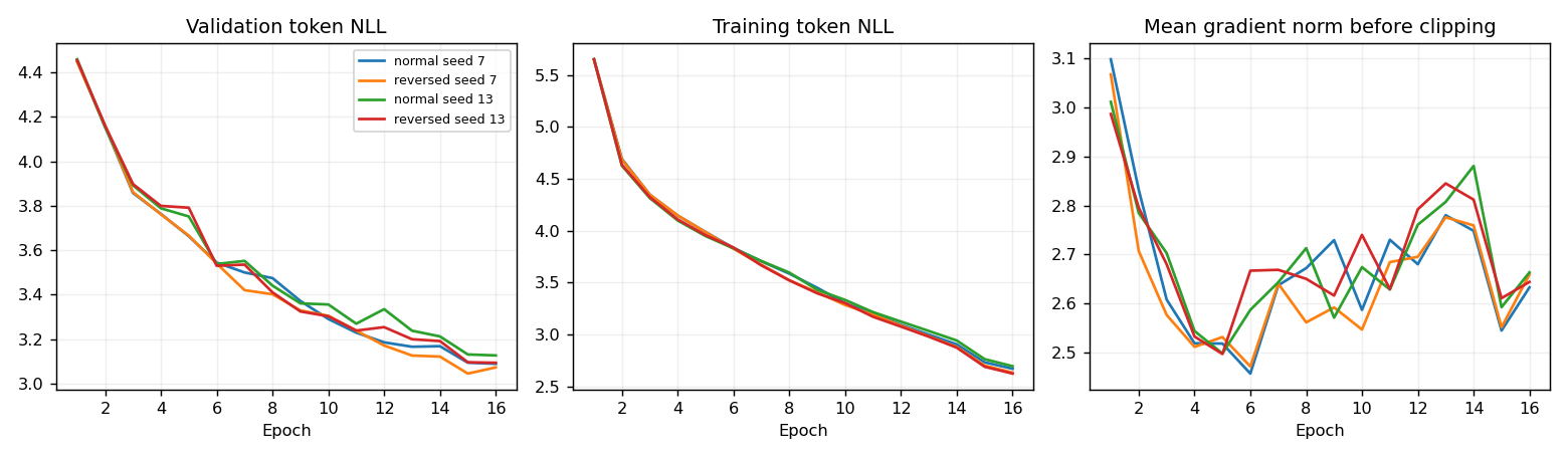
Training uses sentence-averaged token negative log-likelihood, plain SGD, and global gradient clipping at norm 5. Clipping rescales a gradient vector $g$ when its norm exceeds the threshold:

g \leftarrow g \cdot min (1, \frac{5}{∥ g ∥ _{2}}) .

Greedy decoding keeps one best token at every step. Beam search retains several partial hypotheses and ranks them by cumulative log probability. The study evaluates widths 1, 2, 5, and 12 on validation data, then uses the selected width once on the held-out test set.

Experiments and Results

The corpus preparation deterministically samples 2,400 deduplicated Tatoeba English–French pairs and creates a 1,920/240/240 train/validation/test split. Vocabulary construction uses training data only. Two seeds are paired across normal and reversed source order, producing four runs with the same 379,856-parameter architecture and training budget.

Source order	Seed	Selected beam	Test BLEU	Test perplexity
Normal	7	12	2.715	20.619
Reversed	7	5	2.377	19.929
Normal	13	5	1.248	20.811
Reversed	13	5	1.709	19.760

The observed reversed-minus-normal BLEU difference is −0.337 for seed 7 and +0.460 for seed 13, a mean paired difference of only +0.062. With two seeds and a small test set, the evidence does not support a statistical-significance claim.

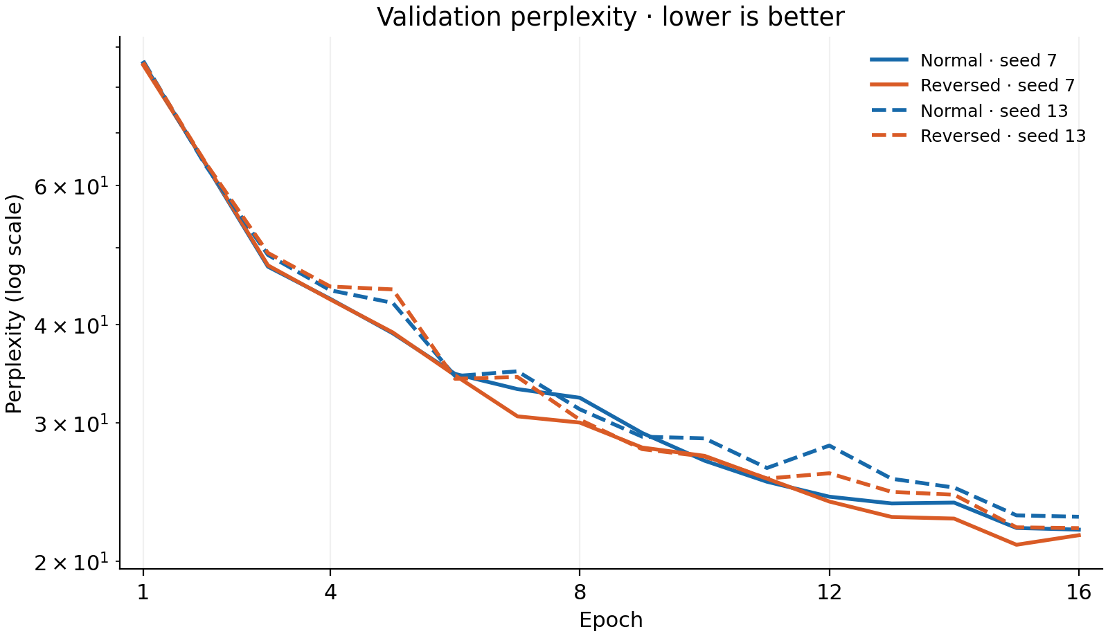
Validation perplexity across the four training runs

BLEU is computed with SacreBLEU on tokenized text. Perplexity is $exp (mean token NLL)$ ; lower values indicate that the model assigns more probability to the reference tokens. Neither metric is directly comparable to the original paper because the dataset, tokenizer, cell variant, model scale, and training budget differ.

What Failed?

The low test BLEU range—1.248 to 2.715—is the central result, not a number to hide. Predictions frequently contain unknown tokens, omit content, or terminate early. For example, the reference for “We talked.” is rendered by one run as “Nous sommes <UNK>.”

The longer-sentence holdout makes the failure sharper. It contains 98 previously unused sentences, including 18 examples with 36 or more source tokens. BLEU falls as low as 0.048 in the longest bucket. Every prediction ended before the decode cap, so the large negative length differences indicate early termination and omission rather than cap truncation.

Source reversal also failed to produce a consistent gain. It can shorten some input-to-output dependency paths, but this experiment cannot isolate that effect from vocabulary limits, optimization variance, and the small training budget.

What I Learned

The implementation supports three evidence-based conclusions:

Correct local mechanics are necessary but not sufficient. Gate parity and gradient checks can pass while translation quality remains poor.
Reproducibility needs more than a seed. Dataset hashes, split hashes, resolved configuration, checkpoint-selection rules, and evaluation signatures all matter.
Negative results become useful when the failure surface is measured. Length buckets, omissions, unknown-token diagnostics, and real predictions explain more than a single aggregate score.

Next Steps

Increase corpus size and training budget before making translation-quality comparisons.
Run more paired seeds and confidence intervals for the source-reversal question.
Add a peephole-cell variant as an isolated architectural comparison.
Reproduce the original tokenization and evaluation protocol before comparing with reported paper scores.
Add attention as a separate experiment to measure how relaxing the fixed-context bottleneck changes long-sentence behavior.